What is machine learning?
Machine learning is often thought to mean the same thing as AI, but they aren’t actually the same. AI involves machines that can perform tasks characteristic of human intelligence. AI can also be implemented by using machine learning, in addition to other techniques.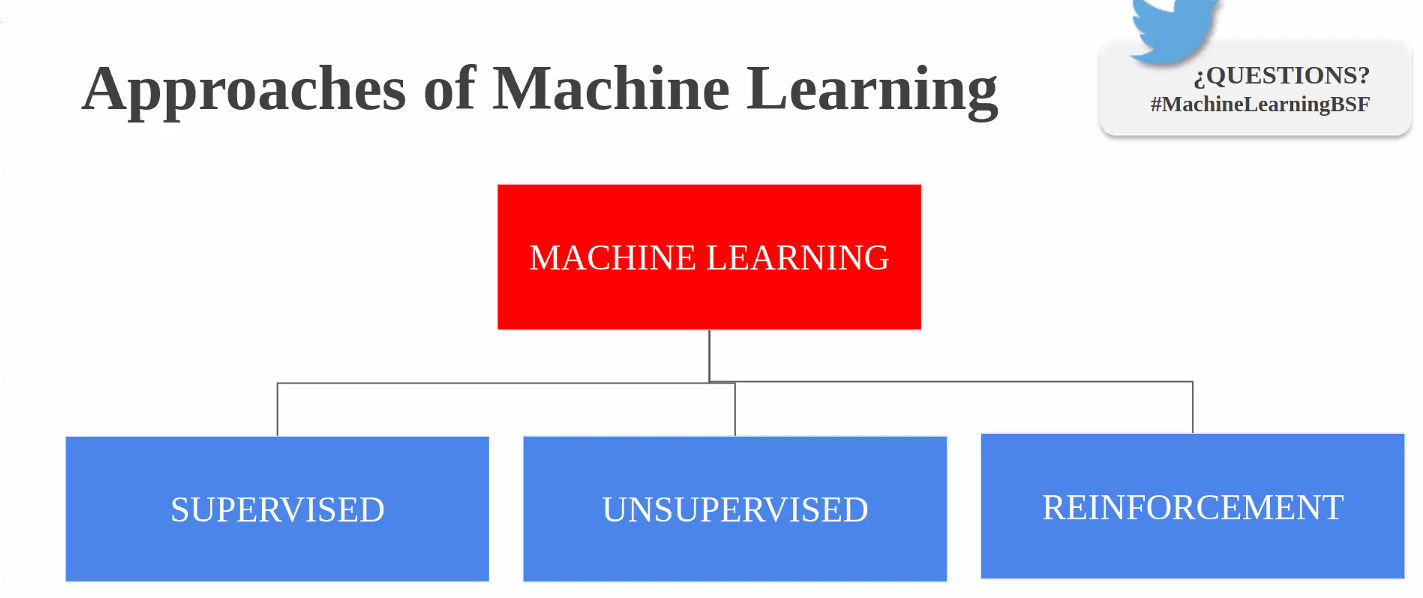
Machine learning itself is a field of computer science that gives computers the ability to learn without being explicitly programmed. Machine learning can be achieved by using one or multiple algorithm technologies, like neural networks, deep learning, and Bayesian networks.
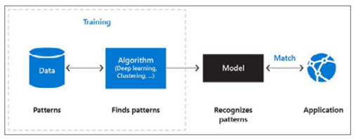
The machine learning process works as follows:
- Data contains patterns. You probably know about some of the patterns, like user ordering habits. It’s also likely that there are many patterns in data with which you’re unfamiliar.
- The machine learning algorithm is the intelligent piece of software that can find patterns in data. This algorithm can be one you create using techniques like deep learning or supervised learning.
- Finding patterns in data using a machine learning algorithm is called “training a machine learning model.” The training results in a machine learning model. This contains the learnings of the machine learning algorithm.
- Applications use the model by feeding it new data and working with the results. New data is analyzed according to the patterns found in the data. For example, when you train a machine learning model to recognize dogs in images, it should identify a dog in an image that it has never seen before.
Visualising datasets
The first step around any data related challenge is to start by exploring the data itself. This could be by looking at, for example, the distributions of certain variables or looking at potential correlations between variables.The problem nowadays is that most datasets have a large number of variables. In other words, they have a high number of dimensions along which the data is distributed. Visually exploring the data can then become challenging and most of the time even practically impossible to do manually. However, such visual exploration is incredibly important in any data-related problem. Therefore it is key to understand how to visualise high-dimensional datasets. This can be achieved using techniques known as dimensionality reduction. This post will focus on two techniques that will allow us to do this: PCA and t-SNE.
https://towardsdatascience.com/visualising-high-dimensional-datasets-using-pca-and-t-sne-in-python-8ef87e7915b
Prepare data
A dataset usually requires some preprocessing before it can be analyzed. You might have noticed some missing values when visualizing the dataset. These missing values need to be cleaned so the model can analyze the data correctly.Basics of Entity Resolution with Python and Dedupe
https://medium.com/district-data-labs/basics-of-entity-resolution-with-python-and-dedupe-bc87440b64d4Categorical columns
- Features which have some order associated with them are called ordinal features.
- Features without any order of precedence are called nominal features.
- There are also continuous features. These are numeric variables that have an infinite number of values between any two values. A continuous variable can be numeric or a date/time.
- For ordinal columns try Ordinal (Integer), Binary, OneHot, LeaveOneOut, and Target. Helmert, Sum, BackwardDifference and Polynomial are less likely to be helpful, but if you have time or theoretic reason you might want to try them.
- For nominal columns try OneHot, Hashing, LeaveOneOut, and Target encoding. Avoid OneHot for high cardinality columns and decision tree-based algorithms.
- For regression tasks, Target and LeaveOneOut probably won’t work well.
https://towardsdatascience.com/smarter-ways-to-encode-categorical-data-for-machine-learning-part-1-of-3-6dca2f71b159
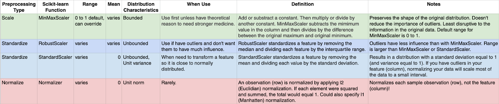
Values normalization
Many machine learning algorithms work better when features are on a relatively similar scale and close to normally distributed. MinMaxScaler, RobustScaler, StandardScaler, and Normalizer are scikit-learn methods to preprocess data for machine learning.https://towardsdatascience.com/scale-standardize-or-normalize-with-scikit-learn-6ccc7d176a02
Synthetic data generation — a must-have skill for new data scientists
A brief rundown of methods/packages/ideas to generate synthetic data for self-driven data science projects and deep diving into machine learning methods.https://towardsdatascience.com/synthetic-data-generation-a-must-have-skill-for-new-data-scientists-915896c0c1ae
https://github.com/tirthajyoti/Machine-Learning-with-Python/blob/master/Synthetic_data_generation/Synthetic-Data-Generation.ipynb?source=post_page---------------------------
Pipeline in Machine Learning with Scikit-learn
Definition of pipeline class according to scikit-learn is “Sequentially apply a list of transforms and a final estimator. Intermediate steps of pipeline must implement fit and transform methods and the final estimator only needs to implement fit.”https://towardsdatascience.com/a-simple-example-of-pipeline-in-machine-learning-with-scikit-learn-e726ffbb6976
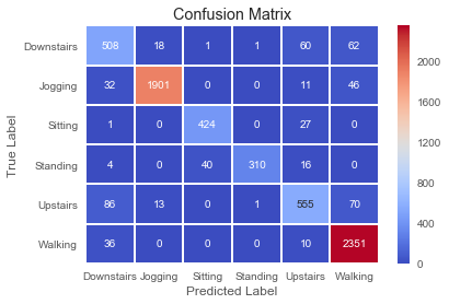
Testing the Neural Network
Precision, recall, and the f1-score
Given the following results:
precision recall f1-score support
0 0.76 0.78 0.77 650
1 0.98 0.96 0.97 1990
2 0.91 0.94 0.92 452
3 0.99 0.84 0.91 370
4 0.82 0.77 0.79 725
5 0.93 0.98 0.95 2397
avg / total 0.92 0.92 0.92 6584
Here is a brief recap of what those scores mean:
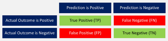
“Prediction versus Outcome Matrix” by Nils Ackermann is licensed under Creative Commons CC BY-ND 4.0
- Accuracy: The ratio between correctly predicted outcomes and the sum of all predictions. ((TP + TN) / (TP + TN + FP + FN))
- Precision: When the model predicted positive, was it right? All true positives divided by all positive predictions. (TP / (TP + FP))
- Recall: How many positives did the model identify out of all possible positives? True positives divided by all actual positives. (TP / (TP + FN))
- F1-score: This is the weighted average of precision and recall. (2 x recall x precision / (recall + precision))
Explainability on a Macro Level with SHAP
The whole idea behind both SHAP and LIME is to provide model interpretability. I find it useful to think of model interpretability in two classes — local and global. Local interpretability of models consists of providing detailed explanations for why an individual prediction was made. This helps decision makers trust the model and know how to integrate its recommendations with other decision factors. Global interpretability of models entails seeking to understand the overall structure of the model. This is much bigger (and much harder) than explaining a single prediction since it involves making statements about how the model works in general, not just on one prediction. Global interpretability is generally more important to executive sponsors needing to understand the model at a high level, auditors looking to validate model decisions in aggregate, and scientists wanting to verify that the model matches their theoretical understanding of the system being studied.https://blog.dominodatalab.com/shap-lime-python-libraries-part-2-using-shap-lime/
Shap explanation and its graphs
https://towardsdatascience.com/interpretable-machine-learning-with-xgboost-9ec80d148d27